Introduction
For performance and cost benchmarks of running OpenMM on SaladCloud, please refer to this blog post. You can also check the GitHub repository for the benchmarking Dockerfile and detailed test methodology. Molecular dynamics simulations with OpenMM can run from several hours to multiple days, depending on factors such as CPU/GPU performance, system size (number of atoms or molecules), simulation length (number of steps), and the level of physical detail modeled. Large-scale simulations often produce substantial output—ranging up to tens of gigabytes—including trajectories and logs. SaladCloud operates on a distributed network of interruptible nodes, meaning any node running your tasks may shut down unexpectedly and all runtime data are removed (data persistence must be managed via external cloud storage). Despite this, most Salad nodes remain stable for over 10 hours at a time. To run OpenMM effectively on SaladCloud, it’s recommended to divide large simulation tasks into manageable chunks—such as 30-minute runs—and execute them sequentially. This chunked approach is natively supported by OpenMM and can be implemented with just a few lines of code. With this adapted workflow, each chunk generates its own small output files and a corresponding checkpoint file, all of which can be uploaded to cloud storage immediately. When resuming after node reallocation, only the input file and the checkpoint file need to be downloaded from the cloud—eliminating the need to upload or download large files at any point. Salad nodes are globally distributed, leading to variations in network latency, geographic distance, and throughput to specific cloud storage endpoints. Many nodes also have asymmetric bandwidth, with upload speeds typically lower than download speeds. Nevertheless, more than 90% of nodes can upload over 10 GB of data per hour—more than sufficient for OpenMM workloads. For detailed performance metrics, refer to the cloud storage benchmarks on SaladCloud.Single-Replica Container Group vs. Job Queue System
As a starting point, we recommend creating a dedicated Single-Replica Container Group (SRCG) for each simulation task on SaladCloud. This setup is easy to launch and works well for larger simulations—spanning tens of hours or multiple days. Task-specific configurations, such as the number of steps, chunking intervals, and input/output paths in cloud storage—can be passed to the instance via environment variables. While tasks are briefly paused during node reallocation after interruptions, our testing across a large number of samples shows that total downtime remains under 4% of the overall runtime. On the other hand, if you’re running a large number of simulation tasks—a job queue becomes essential to ensure efficiency and scalability. Systems like GCP Pub/Sub, AWS SQS, Salad Kelpie, or custom solutions using Redis or Kafka can be used to distribute jobs (task-specific configurations) across a pool of Salad nodes. If a node fails during job execution, the job queue ensures the job is retried immediately on another available node. You can further implement autoscaling by monitoring the number of available jobs in the queue and dynamically adjusting the number of Salad nodes. This approach ensures that your target number of tasks is completed within a defined timeframe, while also allowing cost control during periods of lower demand. This guide focuses on the SRCG-based approach. A separate guide will cover job queue integration.Job Chunking Methodology
To demonstrate how to divide a large OpenMM simulation into manageable chunks, consider the following example. It runs a chunk of 10,000 steps as part of a million-step simulation, downloading two files at the start to resume the state and uploading three files upon completion to back up the state and save the output files.Dynamic Benchmarking and Adaptive Algorithms
OpenMM can only run a chunk for a specified number of steps; it does not support running a chunk based on wall-clock time, such as running each chunk for 30 minutes. A long-running job may be executed sequentially on multiple Salad nodes with different performance characteristics. As a result, running the same number of steps will take varying amounts of time on each node, and if a chunk takes too long, it can lead to greater compute time loss in the event of an interruption. To address this, perform a dynamic benchmark before executing the simulation on a Salad node. For example, running a short test to measure the node’s performance allows us to determine the appropriate number of steps to fit within a 30-minute chunk. Please refer to the example code that implements the workflow described above. It is intended to run on your local machine, without any optimizations for SaladCloud, and supports dynamic benchmarking, simulation interruption and resumption. To use it, you’ll need access to a Cloudflare R2 or other S3-compatible cloud storage bucket and must specify the path of input and output files.Running OpenMM on SaladCloud
Code Optimizations
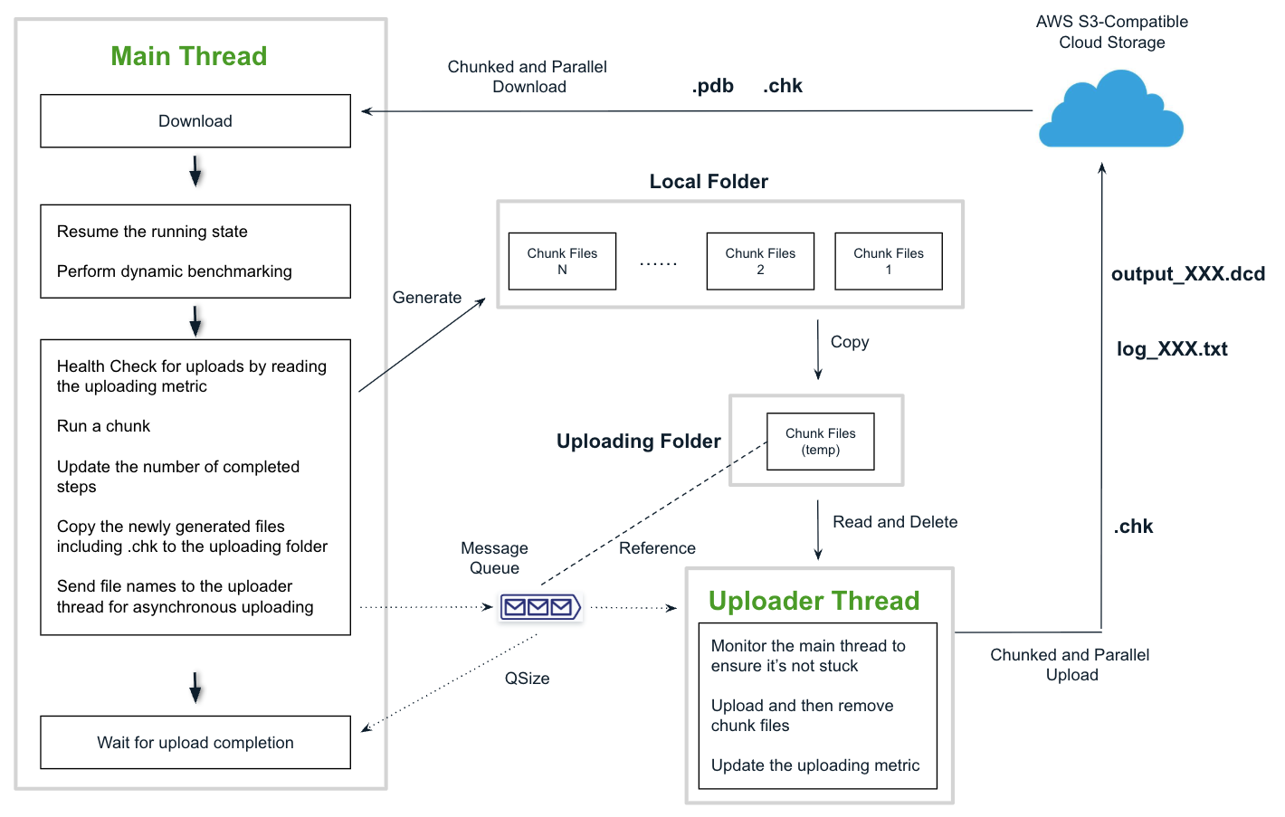
To run OpenMM efficiently on SaladCloud, several additional code optimizations are recommended:- Use chunked and parallel data transfers to maximize throughput when uploading or downloading large files between Salad nodes and cloud storage.
- Introduce a dedicated uploader thread with task queue to offload upload operations from the main thread, ensuring that simulation execution remains unblocked.
- Add error handling, monitoring, and logging to improve reliability, enhance visibility, and simplify troubleshooting.
Dockerfile Configuration
The provided Dockerfile creates a containerized environment by using the miniconda official image, then installing essential utilities (VS Code Server CLI), OpenMM 8.3.0 and required dependencies. It copies the required Python code into the image and sets the default command.Environment Variables
Ensure all required environment variables are set before running a simulation. These variables will be passed to the SRCG at creation time. For easy configuration and reuse, you can define them in a .env file located in the project directory..env
Local Run
If you have access to a local GPU environment, you can perform a test of the image before running it on SaladCloud. Usedocker compose to start the container defined in
docker-compose.yaml. The command
automatically loads environment variables from the .env file in the same directory.